Foodhub data analysis

mailfreda
Aug 21, 2025
5 min read

Project Python Foundations

Link to code:

Data_Analysis_Projects/Foodhub_data_analysis_and_recommendations (2).ipynb at main · FredaMaree/Data_Analysis_Projects

Objective: The food aggregator company has stored the data of the different orders made by the registered customers in their online portal. Analyze the data to get a fair idea about the demand of different restaurants which will help them in enhancing their customer experience.

Loading the dataset

# Return first 5 rows foodhub.head()

	order_id	customer_id	restaurant_name	cuisine_type	cost_of_the_order	day_of_the_week	rating	food_preparation_time	delivery_time
0	1477147	337525	Hangawi	Korean	30.75	Weekend	Not given	25	20
1	1477685	358141	Blue Ribbon Sushi Izakaya	Japanese	12.08	Weekend	Not given	25	23
2	1477070	66393	Cafe Habana	Mexican	12.23	Weekday	5	23	28
3	1477334	106968	Blue Ribbon Fried Chicken	American	29.20	Weekend	3	25	15
4	1478249	76942	Dirty Bird to Go	American	11.59	Weekday	4	25	24

Understanding the data

# Amount of rows and columns in the dataset

foodhub.shape

(1898, 9)

# Datatypes of the different columns in the dataset

foodhub.info()

<class 'pandas.core.frame.DataFrame'>
RangeIndex: 1898 entries, 0 to 1897
Data columns (total 9 columns):
 #   Column                 Non-Null Count  Dtype  
---  ------                 --------------  -----  
 0   order_id               1898 non-null   int64  
 1   customer_id            1898 non-null   int64  
 2   restaurant_name        1898 non-null   object 
 3   cuisine_type           1898 non-null   object 
 4   cost_of_the_order      1898 non-null   float64
 5   day_of_the_week        1898 non-null   object 
 6   rating                 1898 non-null   object 
 7   food_preparation_time  1898 non-null   int64  
 8   delivery_time          1898 non-null   int64  
dtypes: float64(1), int64(4), object(4)
memory usage: 133.6+ KB

Findng missing values and treating it

# Rating is recorded as an object, because "not given" is entered as a string foodhub['rating'].unique()

array(['Not given', '5', '3', '4'], dtype=object)

# Change rating to a float
foodhub['rating']=foodhub['rating'].replace('Not given', np.nan)
foodhub
foodhub['rating']=foodhub['rating'].astype(float)

Getting statistical summary of numerical data

# Statistical summary of the numerical data # Drop customer id and order id columns, they contain numbers, but are not numerical values

foodhub.drop(['customer_id', 'order_id'], axis=1).describe()

	cost_of_the_order	rating	food_preparation_time	delivery_time
count	1898.000000	1162.000000	1898.000000	1898.000000
mean	16.498851	4.344234	27.371970	24.161749
std	7.483812	0.741478	4.632481	4.972637
min	4.470000	3.000000	20.000000	15.000000
25%	12.080000	4.000000	23.000000	20.000000
50%	14.140000	5.000000	27.000000	25.000000
75%	22.297500	5.000000	31.000000	28.000000
max	35.410000	5.000000	35.000000	33.000000

Observation: The average preparation time is 27.37 minutes. The minimum preparation time is 20 minutes and the maximum preparation time is 35 minutes.

The delivery time ranges from 24 to 33 minutes, with an average of 24 minutes.

Rating has a count of 1162, which indicates missing values in this column.

Obtaining orders that are not rated

df=pd.DataFrame(foodhub)

#Sum Nan values

nan_counts=df.isnull().sum() print(nan_counts)

order_id                   0
customer_id                0
restaurant_name            0
cuisine_type               0
cost_of_the_order          0
day_of_the_week            0
rating                   736
food_preparation_time      0
delivery_time              0
dtype: int64

Exploratory Data Analysis: Univariate Analysis

Observation on Customer ID

# Count of customer ID numbers

foodhub['customer_id'].nunique()

Observation: There are 1200 unique customer ID numbers. This indicates that some of the customers ordered more than once.

Observation on the Restaurant name

# Explore the variable of restaurant names

foodhub['restaurant_name'].unique()

foodhub['restaurant_name'].nunique()

There are 178 restaurants

Observation on Cuisine types
# Countplot for cuisine type
plt.figure(figsize=(15,5))
sns.countplot(data=foodhub, x= 'cuisine_type');
plt.xticks(rotation=90);
plt.xlabel('Cuisine type');
plt.ylabel('Count');
plt.title('Cuisine type');
plt.show()
     
American, Japanese, Italian and Chinese are the top ordered cuisines.



#Cost of orders
#Boxplot for cost of order
sns.boxplot(data=foodhub,x='cost_of_the_order');
plt.xlabel('Cost of order');
plt.ylabel('Count');
plt.title('Distribution of cost of orders');
plt.show()

Observation: Distribution of cost of orders: The cost of the order ranges between a minimum of 4.5 dollar and a maximum of 35.41 dollar with an average amount of 16.5 dollar. The median price is 14 dollar. The pattern is skewed to the right and no outliers are seen.

#Distribution of food preparation time:

The food preparation time is almost evenly distributed with a minimum of 20 minutes and a maximum time of 35 minutes. T

Top 5 restaurants in terms of the number of orders received

# Creating a DataFrame

df = pd.DataFrame(foodhub)

# Count number of orders per restaurant

restaurant_order_count = df['restaurant_name'].value_counts().head(5),

# Display Top 5 restaurants

print(restaurant_order_count)

(restaurant_name
Shake Shack                  219
The Meatball Shop            132
Blue Ribbon Sushi            119
Blue Ribbon Fried Chicken     96
Parm                          68
Name: count, dtype: int64,)

Most popular cuisine on weekends

# Determine most popular cuisine type over the weekend

sns.countplot(data=foodhub, x= 'cuisine_type', hue= 'day_of_the_week'); plt.xticks(rotation=90); plt.xlabel('Cuisine type'); plt.ylabel('Count'); plt.title('Cuisine type by day of the week');

plt.show()

Observation: The most popular cuisine type over weekends is American with count of 415, followed by Japanese with a count of 335.

Mean order delivery time

# Total order delivery time for the column

total_delivery_time= foodhub['delivery_time'].sum()

total_delivery_time

# Mean order delivery time mean_order_delivery_time= total_delivery_time/1898 rounded_percentage= round(mean_order_delivery_time,2)

print('The mean order delivery time is:',rounded_percentage,'minutes')

The mean order delivery time is: 24.16 minutes

Exploratory Data Analysis: Multivariate analysis

Correlation by heatmap

#Multivariate analysis, evaluating numerical data

#Set the correlation matrix corr_matrix=foodhub[['cost_of_the_order','rating','food_preparation_time','delivery_time', ]].corr()

# Create heatmap sns.heatmap(data=corr_matrix, annot=True, cbar=True,cmap='bwr',vmin=-1, vmax =1)

plt.title('Correlation heatmap');

plt.show()

Observation: The heatmap shows correlation between numerical values. There is a weak positive correlation between cost of order and food preparation time (0.042). There is almost no correlation between rating and food preparation time,rating and delivery time or rating and cost of order.

Multivariate analysis by pairplot

sns.pairplot(data=foodhub[['cost_of_the_order','rating','food_preparation_time','delivery_time', 'total_delivery_time']]);

plt.show()

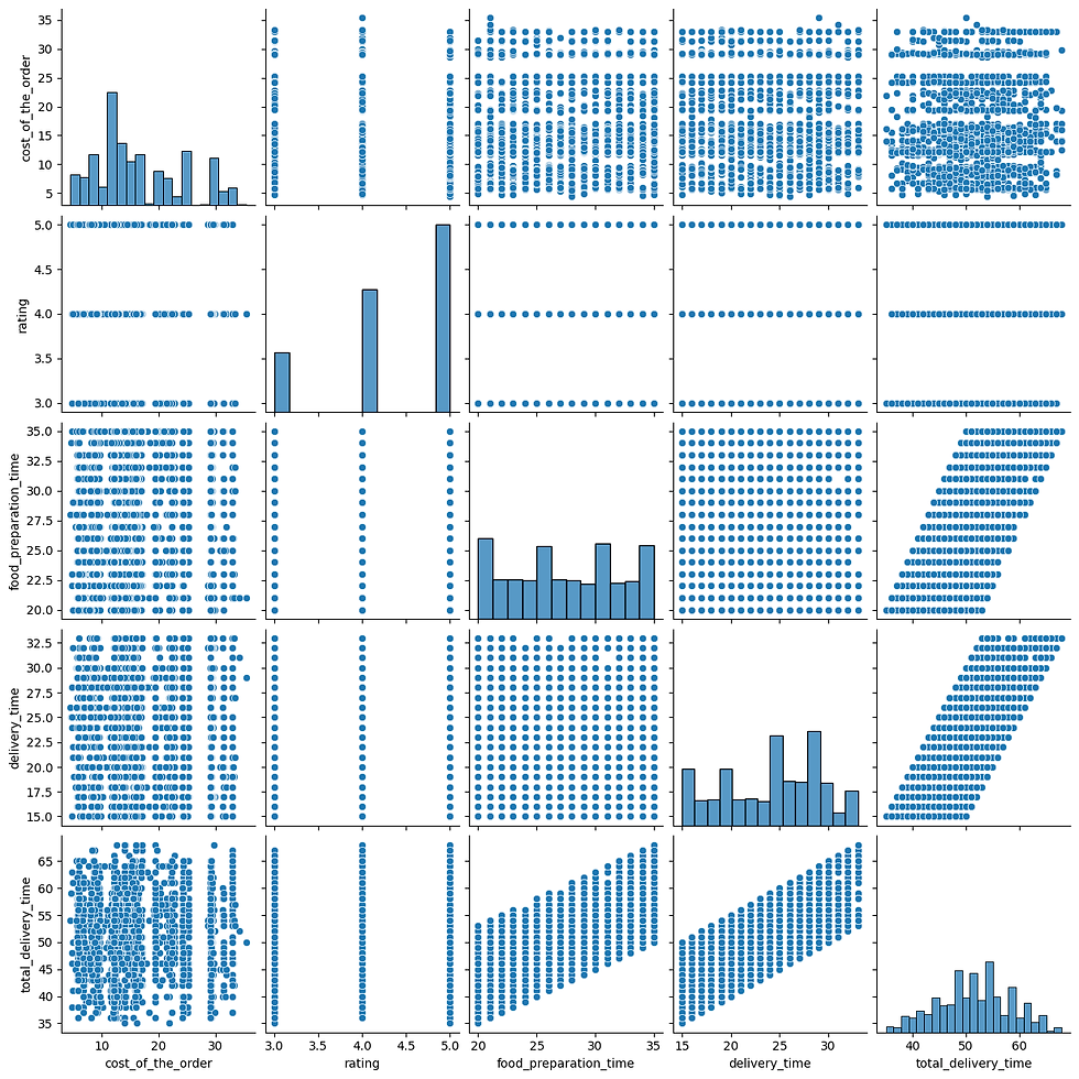
This can also be seen in the pairplot and here a strong correlation is present between food preparation time and total delivery time, as well as delivery time and total delivery time as expected.

Net revenue generated across all orders

def calculate_revenue(cost_of_the_order):

""" Calculate revenue based on the cost of the order. Revenue is determined by the following conditions: - 25% of the cost if cost_of_the_order > 5

- 0% of the cost if cost_of_the_order <= $5 """

if cost_of_the_order > 20: revenue = cost_of_the_order 0.25

elif cost_of_the_order > 5: revenue = cost_of_the_order 0.15

else: revenue = cost_of_the_order * 0

return revenue

# Apply the revenue calculation to the 'cost_of_the_order' column

df['revenue'] = df['cost_of_the_order'].apply(calculate_revenue)

print(df)

# Apply the function to the 'cost_of_the_order' column and create a new 'revenue' column foodhub['revenue'] = foodhub['cost_of_the_order'].apply(calculate_revenue) print(foodhub)

#Calculate total revenue total_revenue = foodhub['revenue'].sum()

print('Total Revenue is ',round(total_revenue,2), 'dollars')

Total Revenue is 6166.3 dollars

Business insights:

Customers show the highest satisfaction with American and Italian cuisines, and overall ratings average 4.3 despite nearly 39% missing data. Revenue is skewed by higher-value orders, delivery is quicker on weekends, and top-performing restaurants and loyal customers drive consistent business, while delivery time shows no clear link to customer ratings.

Recommendations:

Focus on promoting top-rated cuisines, improving weekday delivery efficiency, increasing customer feedback, boosting underperforming cuisine types, and introducing customer reward programs to drive growth and satisfaction.